第 2 章 - Basic Simulation Template
來源 PDF 頁碼: 7-24
目錄
- 2.1 Simulation flow 介紹
- 2.2 Layout Setup
- Material
- Roughness
- Etching
- Stackup 資訊更新
- 2.3 Simulation Setup
- Automatic port setup
- Manual port setup
- Multi-Terminal Circuits
- 2.4 Clarity 3D Layout Simulation Options
- Frequency Settings
- Solver Options
- Geometry Options
- 2.5 Cut-Stitch Options
- 2.6 Simulation
- 2.7 View, Check, Process Result
2.1 Simulation flow 介紹
Cadence 已在 Clarity 3D Layout 左側 workflow pane 中整理 simulation flow。後續各節依此順序設定 Layout Setup、Simulation Setup、Clarity 3D Layout Simulation Options、Cut-Stitch Options 與 Simulation。
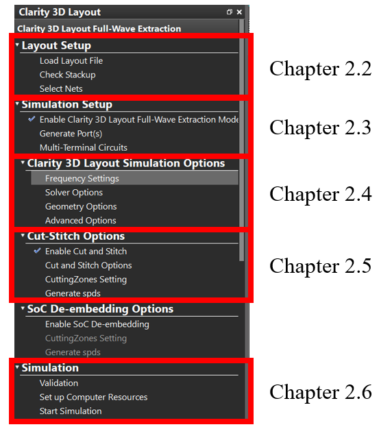
圖 2.1.1:Clarity 3D Layout workflow pane
為方便後續描述,本文件使用下圖中的 UI 區域名稱,例如 Workflow Pane、Top Tool Bar、Right Tool Bar 與 Command Sheet。
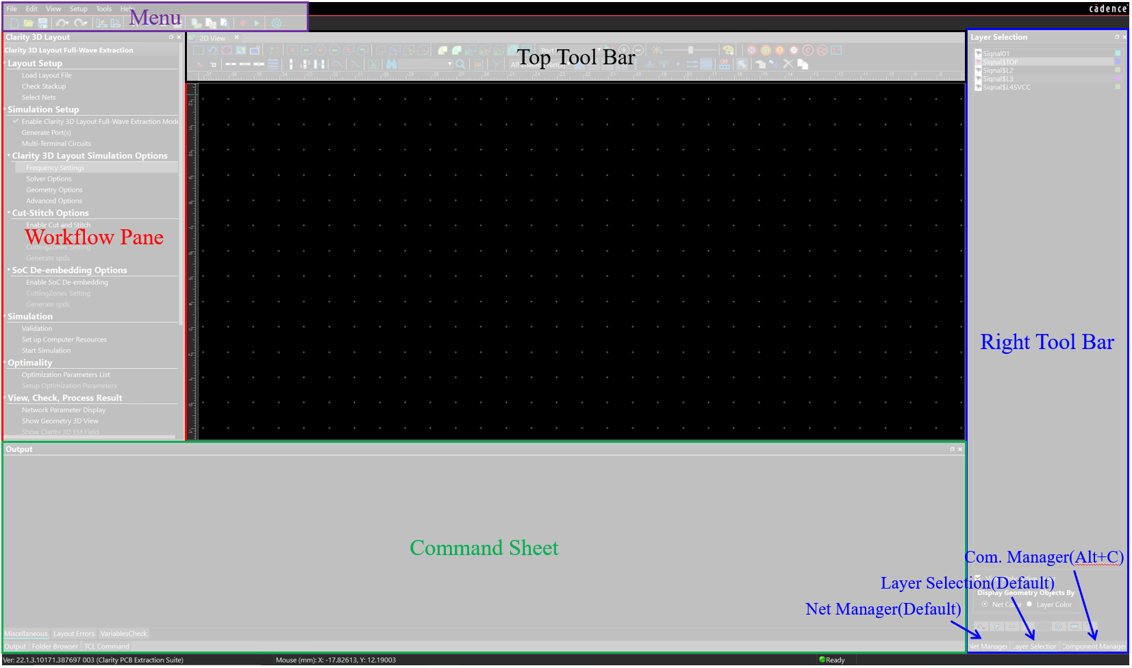
圖 2.1.2:Clarity 3D Layout UI 區域定義
2.2 Layout Setup
由於 Allegro PCB viewer / editor 與 Clarity 同屬 Cadence flow,Clarity 3D Layout 可直接匯入 .brd layout file。
- 開啟
Clarity 3D Layout。 - 選擇
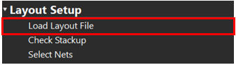
Load Layout File,載入要進行 simulation 的 layout。
- 快速確認 model geometry 是否正確。
- 在執行
Check Stackup前,先建立本次 simulation 需要的 material、roughness 與 etching 設定。
2.2.1 Material
依序執行:
Check Stackup > 勾選 Enforce Causality > View Material > 選擇 D-Sarkar Model
接著:
- 在
*旁直接輸入新的 material name 建立材料。 - 在右側選擇
Dielectric。 - 輸入對應的
Freq/DK/DF。
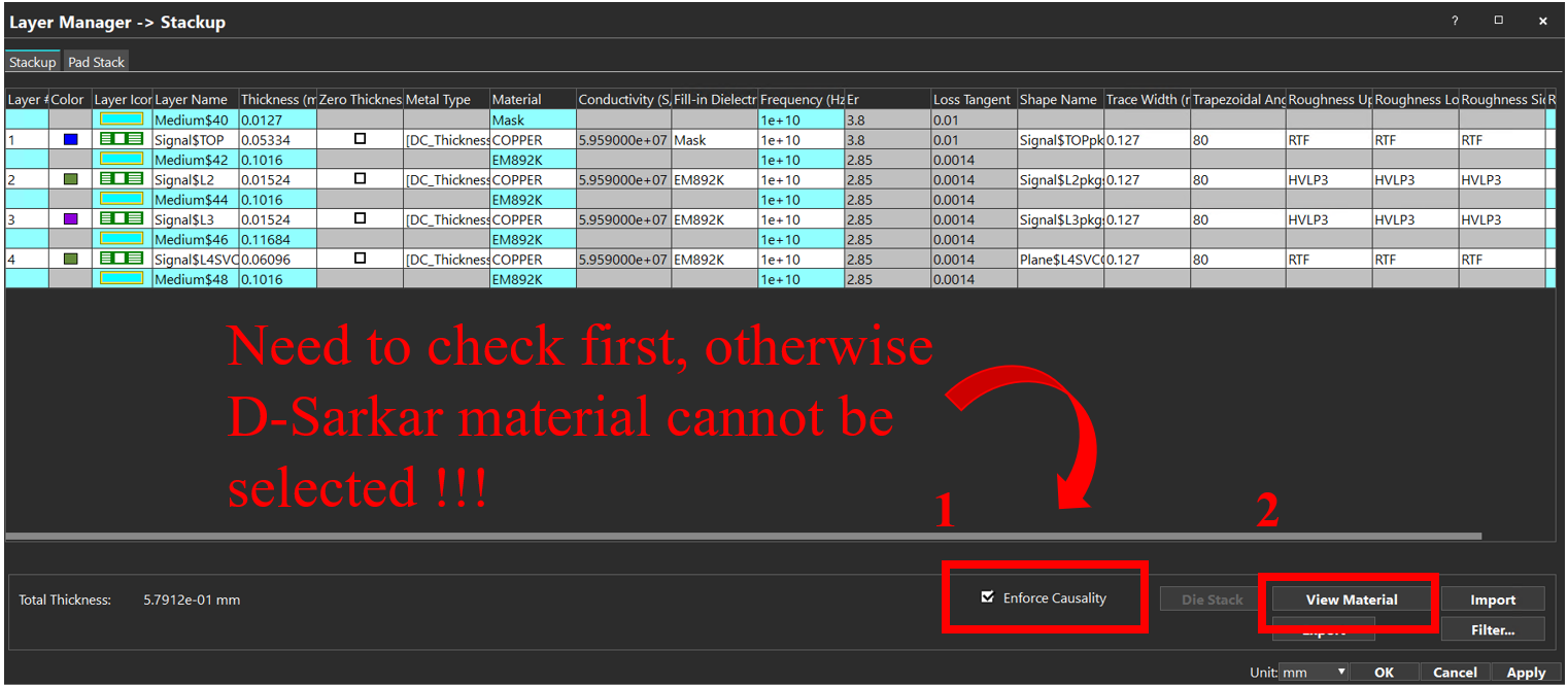
圖 2.2.2:在 stackup 中先啟用 `Enforce Causality`
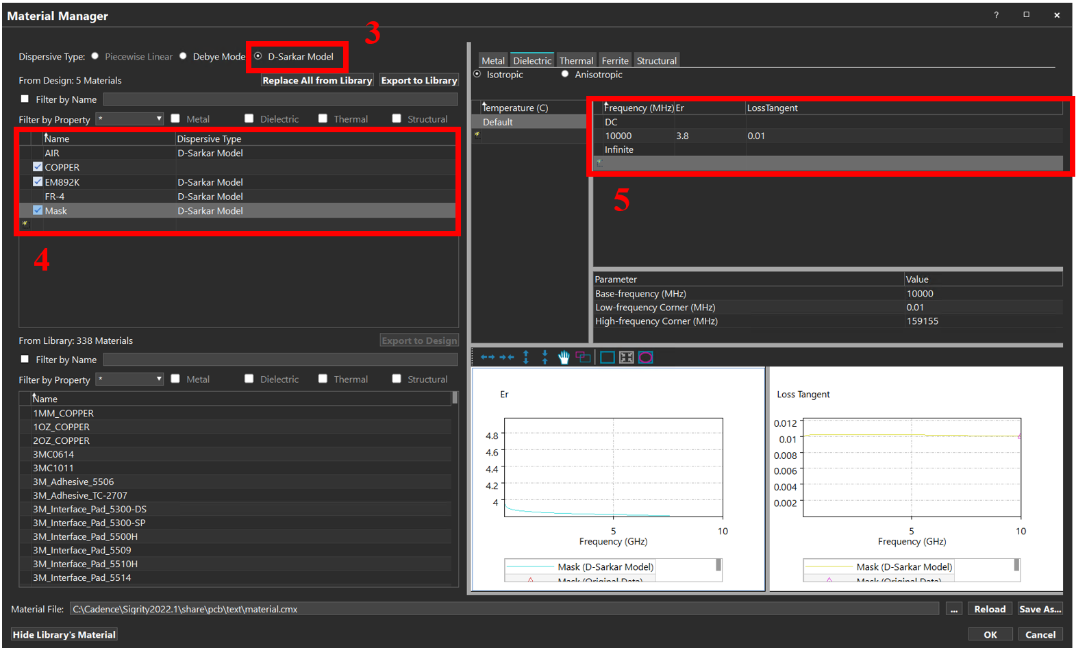
圖 2.2.3:以 D-Sarkar Model 建立 dielectric material
2.2.2 Roughness
從 top menu 選擇:
Edit > Surface Roughness Library > Add Huray Model
建立 row 後 double-click parameter value,依來源文件設定:
| Parameter | Source setting |
|---|---|
Surface Ratio |
4.9 |
Snowball Radius |
0.06 × Rz(um) |
來源提供的 Rz reference 如下:
| Material | Rz (um) |
|---|---|
| HTE | 8 |
| RTF | 3.5 |
| RTF2 | 3 |
| RTF3 | 2.5 |
| VLP | 3 |
| HVLP | 2 |
| HVLP2 | 1.5 |
| HVLP3 | 1 |
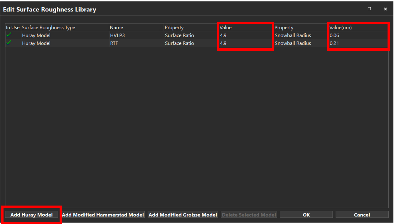
圖 2.2.4:Surface Roughness Library 的 Huray Model 設定
2.2.3 Etching
在 Layer Manager-Stackup 中直接輸入 Trapezoidal Angle。來源畫面指出,可在 Clarity 3D Workbench 觀察 model angle,作為 <90、=90、>90 的設定參考。
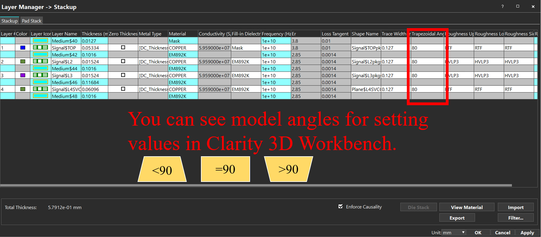
圖 2.2.5:`Trapezoidal Angle` 設定
2.2.4 Stackup 資訊更新
完成 material / roughness / etching 後,回到 Check Stackup,將各 layer 資訊修改為 design value。來源提供兩種方法。
方法 A - 直接修改
- 開啟
Check Stackup。 - 在表格中直接輸入各 layer value。
- 按
OK。
方法 B - 使用 CSV 編輯
- 在
Check Stackup選擇Export。 - 以 Microsoft Excel 編輯輸出的
.csvfile。 - 回到 server / stackup flow,選擇
Import。 - 載入修改後的
.csvfile。 - 按
OK。
2.3 Simulation Setup
本 basic flow 以 Lump port 為主要 port setup。來源文件將 port setup 分為 Automatic 與 Manual 兩種方式。
2.3.1 Automatic port setup
Automatic flow 可依 component 建立 port。
- Enable 需要的 net;最後的 port 數量會依 enabled network / net 數量而定。
- 選擇
Generate Port(s)。
- 選擇
Coaxial Port。 - 選擇 component layer 與 model name。
- 依序按
Next>Next(default)>Finish(default)。
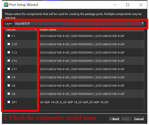
圖 2.3.2:選擇 component layer 與 model name
完成後可在 Port window 檢查 generated ports。
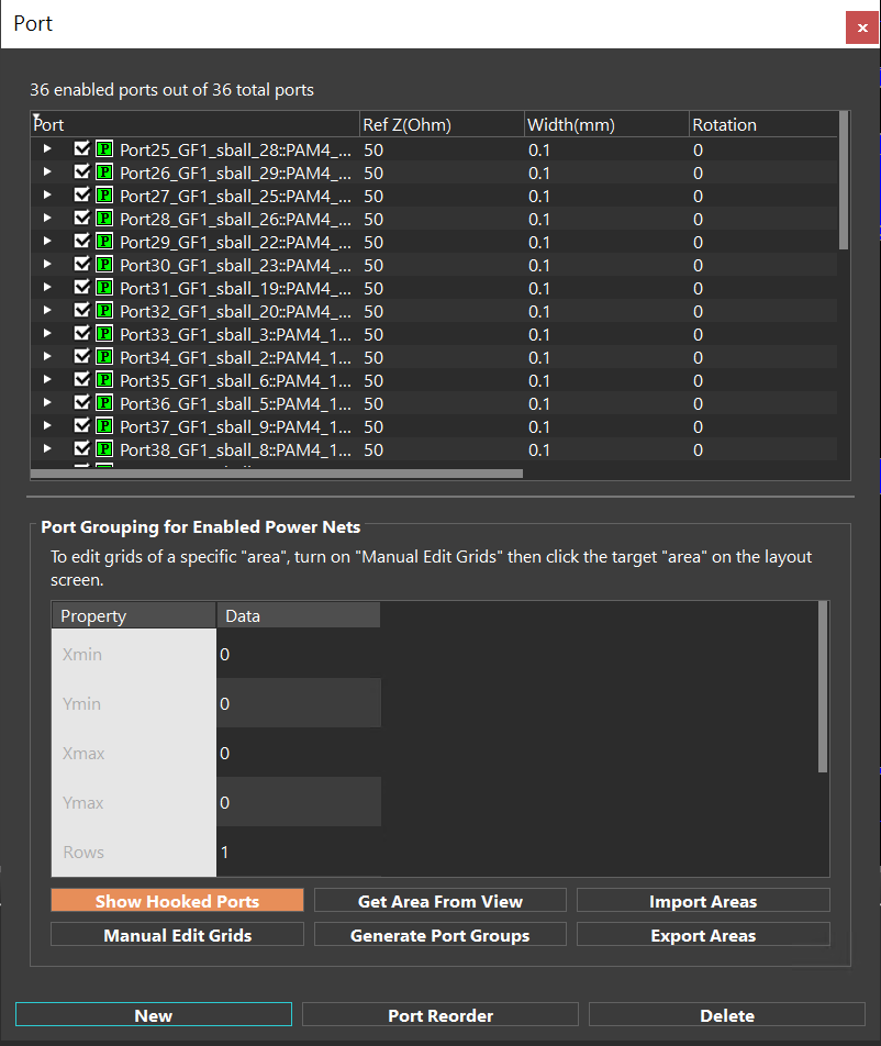
圖 2.3.3:Port 產生完成後的清單
2.3.2 Manual port setup
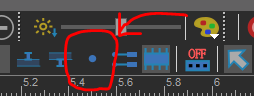
Manual flow 可在 node 與 node 之間建立 port。要選取 node 前,先在 top tool bar 切換為 Select Node。
建立 vertical Lump port 的操作如下:
- 在 top tool bar 選擇
Add Node。 - 點選要新增 node 的位置與 layer。
- 選擇
Setup>Port>New。 - 在 Port window 選取要設定的 port,該 port 必須保持 highlight。
- 對 signal node 按右鍵並選擇
Hook+。 - 對 GND node 按右鍵並選擇
Hook-。
若 trace 原本已經有可用 node,可直接使用,不必額外建立新 node。
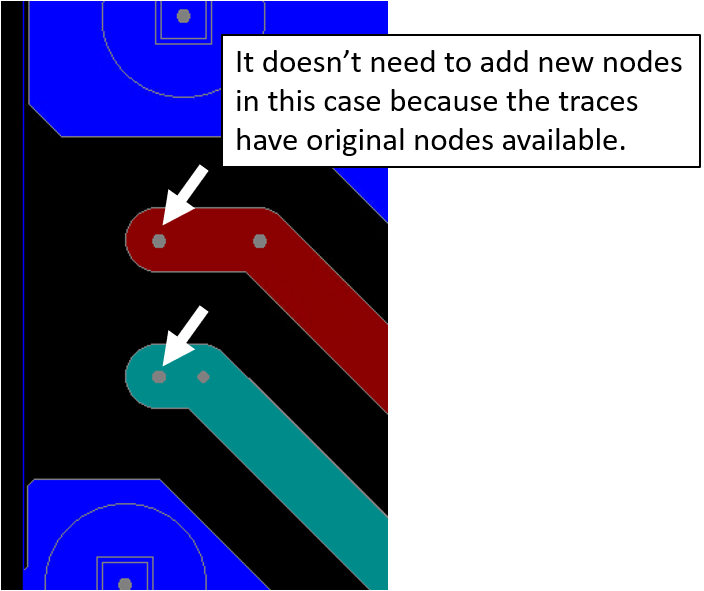
圖 2.3.4:建立或使用既有 node
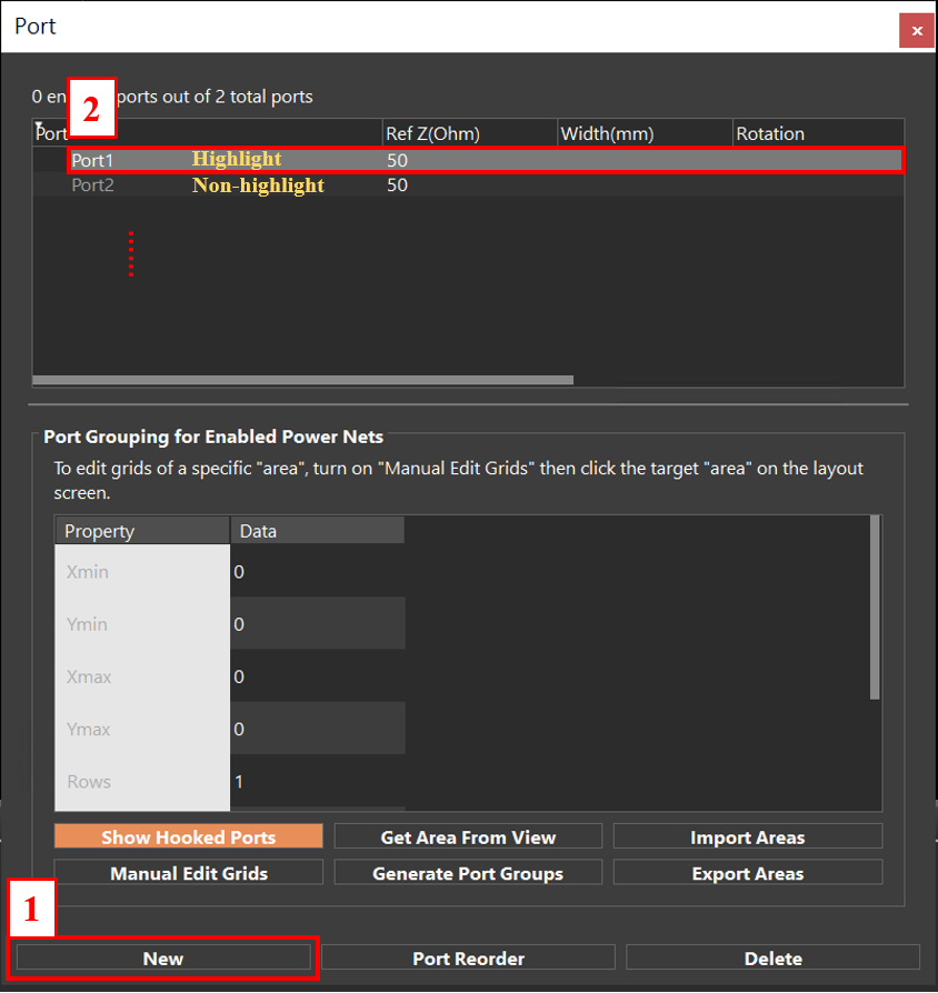
圖 2.3.5:建立新的 Port
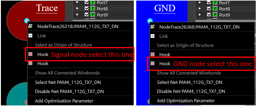
圖 2.3.6:Signal node 與 GND node 的 Hook 設定
2.3.3 Multi-Terminal Circuits
若 signal path 上存在 component,需設定 Multi-Terminal Circuits;若 signal path 沒有 component,可略過此步驟。
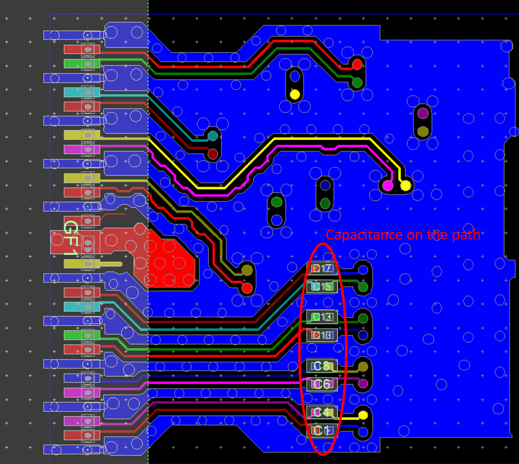
圖 2.3.7:Signal path 上的 E-load / component
要修改 component definition:
- 按
Alt+C開啟右側Component Manager。 - 選擇目標 component 並編輯 model。
- 來源示範將 capacitor 改為 resistor,definition 設為
R 1 2 0;其含義為 node 1 到 node 2 為 short circuit。
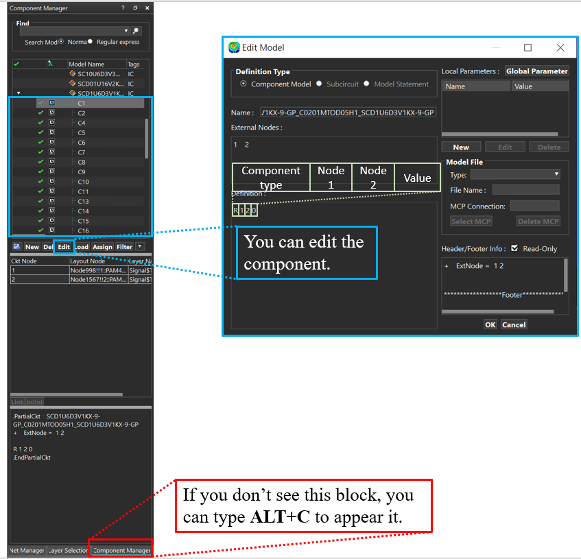
圖 2.3.8:Component Manager 與 component model 編輯
完成 component setting 後:
Multi-Terminal Circuits > Multi-Terminal Circuits Setting > 勾選 signal path 上需要處理的 component > OK
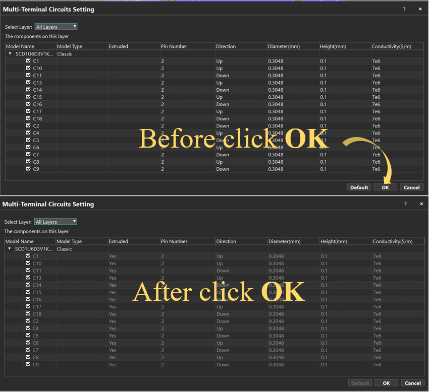
圖 2.3.9:Multi-Terminal Circuits 設定前後
來源畫面亦比較 Circuit Setting 前後的 Component Manager 狀態。
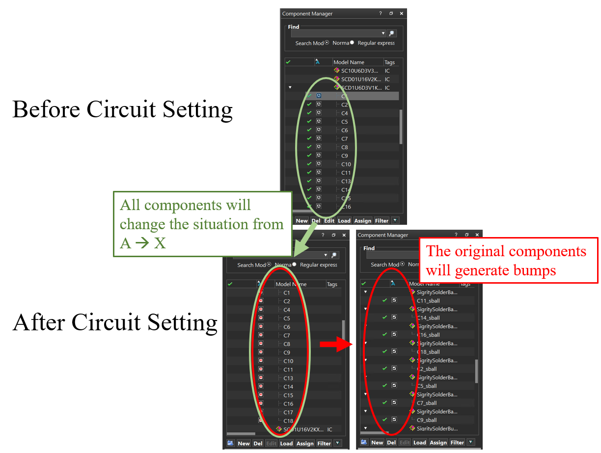
圖 2.3.10:Circuit Setting 前後的 Component Manager 狀態
2.4 Clarity 3D Layout Simulation Options
2.4.1 Frequency Settings
在 workflow pane 選擇 Frequency Settings。
Solution frequency
可輸入多個 solution frequency,各 frequency 之間以空白分隔,例如:
1e+8 3e+10 6e+10
來源文件不建議設定多個 solution frequency,理由是 simulation time 會增加,而文件所觀察到的結果差異不明顯。
Frequency sampling
| Parameter | 說明 |
|---|---|
Fmin(Hz) |
Frequency sweep 的 minimum frequency |
Fmax(Hz) |
Frequency sweep 的 maximum frequency |
Sampling Mode |
可選 Linear、Log、Single Point;default 為 Linear |
Step(Hz) |
Linear sampling mode 的 step size |
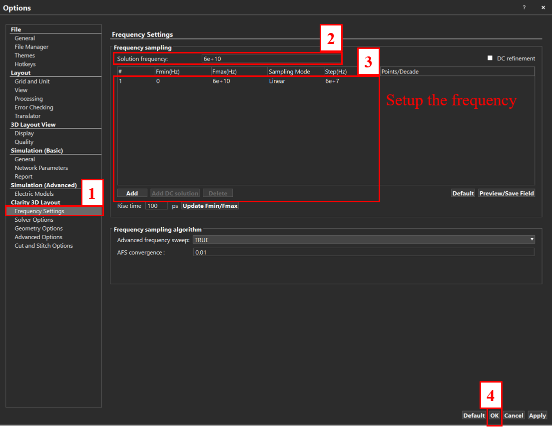
圖 2.4.1:Frequency Settings
2.4.2 Solver Options
在 workflow pane 選擇 Solver Options。來源文件提供以下 recommended settings:
| Parameter | Source recommendation | Source rationale |
|---|---|---|
Metal type |
DC_Thickness |
與 Auto_Fitting 結果相近,但可縮短 simulation time |
Basis function order |
MIXED FS |
可明顯降低 frequency sweep runtime,來源認為結果差異很小 |
Target delta S |
0.02 |
值越小,accuracy 越高 |
Min number of converged iterations |
2 |
值越大,accuracy 越高 |
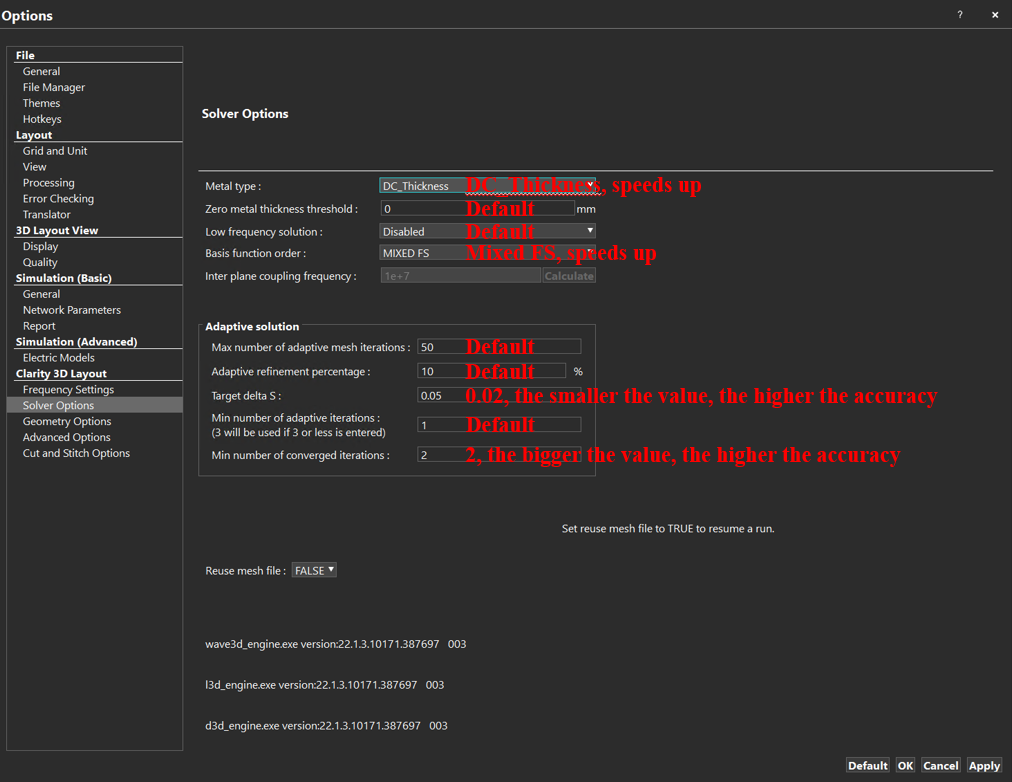
圖 2.4.2:Solver Options
2.4.3 Geometry Options
在 workflow pane 選擇 Geometry Options。
| Parameter | Source recommendation / 說明 |
|---|---|
Number of points |
用於 cylindrical object modeling,建議 6 ~ 8 |
Outer box buffer size |
dx+ / dx- / dy+ / dy- 建議設為 0;或勾選 Use conformal outer box |
Mesh |
DMesh、XMesh、LMesh;來源速度排序為 LMesh (unpublished) > XMesh (unstable) > DMesh (default) |
來源建議可先嘗試 XMesh;若出現 mesh 相關 error code,再切回 DMesh。
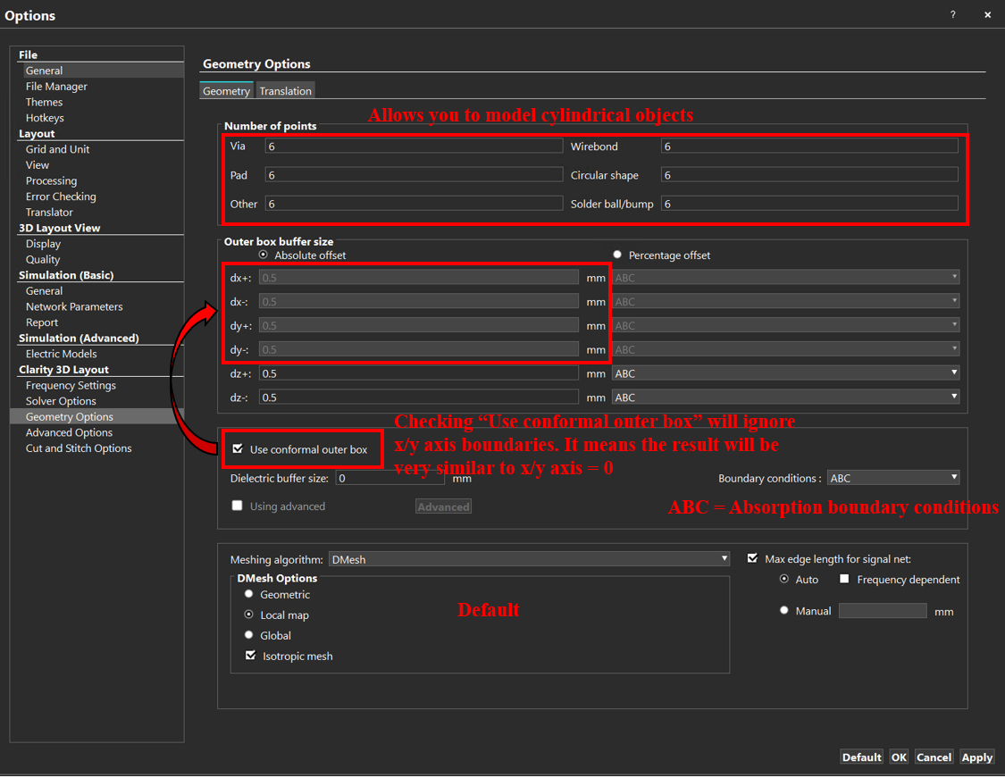
圖 2.4.3:Geometry Options
2.5 Cut-Stitch Options
若 simulation area 不大且不複雜,可略過 Cut-Stitch setup。來源文件指出需要 cut 時應參考 Chapter 3。
來源內容缺口: Chapter 3.1
Cut and Stitch在原 PDF 中只有 section title,沒有提供進一步 procedure。
2.6 Simulation
完成 basic settings 後,先使用 Validation 檢查 setup,再設定 computer resources 並開始 simulation。
- Validation:直接點選
Validation,確認沒有 error code。 - Set up Computer Resources:來源示範 CPU 數量設定為
8;實際可用 CPU 取決於 license / resource。 - Start Simulation:點選
Start Simulation。
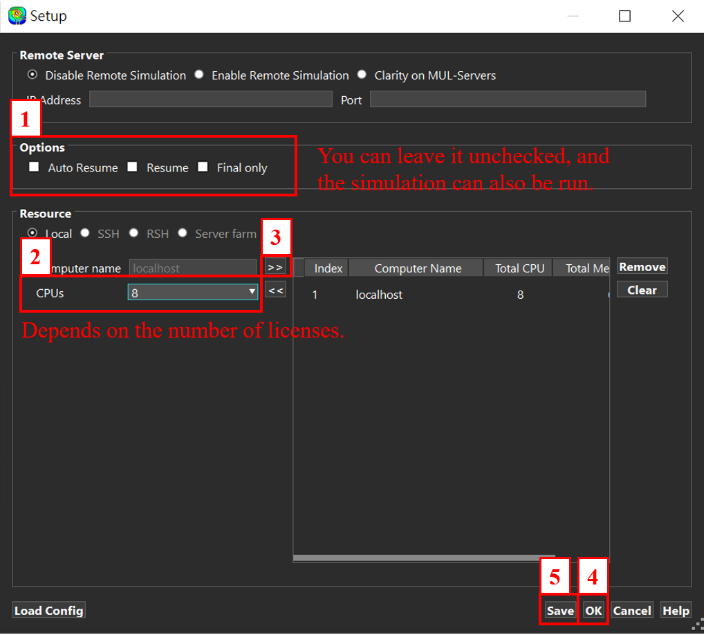
圖 2.6.1:Set up Computer Resources
Auto Resume、Resume 與 Final Only 的用途請參考 第 4 章 - Computer Resources Options。
2.7 View, Check, Process Result
2.7.1 Load SNP file
可透過 Network Parameter Display 載入 SNP file 檢查結果。若是剛完成的 simulation,result 通常可直接顯示,不一定需要重新 load。
操作路徑:
Network Parameter Display > 在 Network Parameters 按右鍵 > Load > 選擇 SNP file
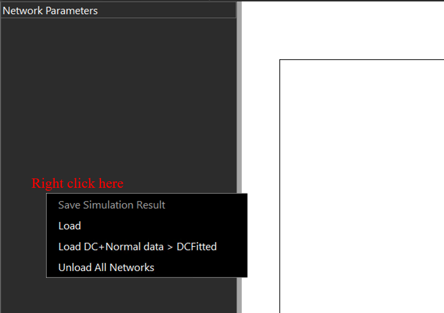
圖 2.7.1:載入 SNP file
2.7.2 Define Differential Pair
需要建立 differential representation 時:
- 對 SNP file title 按右鍵。
- 選擇
Matrix Operations>Redefine Differential Port...。 - 設定 P/N net 與對應 port。
- 按
Add Pair。 - 按
OK。 - 切換至
Differential Channel View。 - Double-click 目標 plot,可放大檢視。
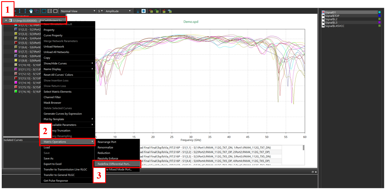
圖 2.7.2:由 Matrix Operations 進入 differential port 定義
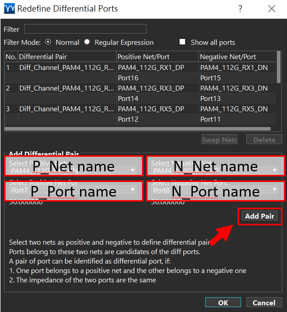
圖 2.7.3:設定 P/N net 與 port
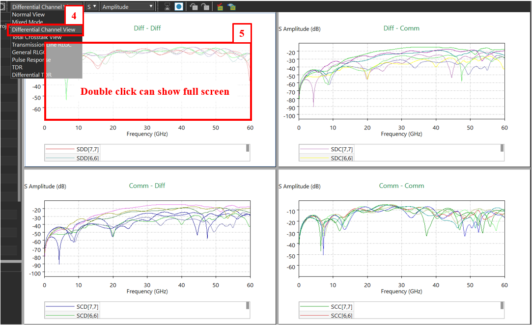
圖 2.7.4:Differential Channel view
2.7.3 Simulation Results Checking Tools
來源畫面列出幾個常用檢查方式:
- 調整 X/Y scale。
- 對 curve 按右鍵修改 line property。
- Double-click plot title 進行 title 編輯。
- 在 plot 上按右鍵使用
Marker/ measurement 功能。
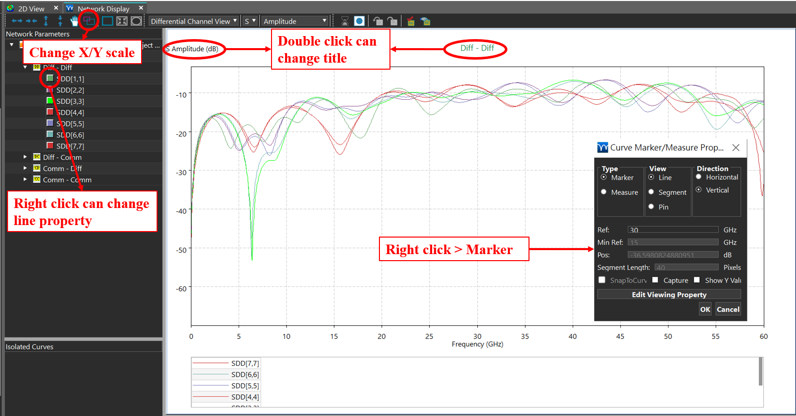
圖 2.7.5:Simulation result 常用檢查工具